Plotting and Saving

One of the main benefits of ParticleSpy is the ability to plot particle properties natively. The main method for plotting particle properties is plot(). This method plots either a histogram of any specified property or a scatter plot of two properties, as long as you have added these properties to each particle (either automatically or manually).

An example of plotting a histogram of particle areas in shown here:

>>> particles = ps.particle_analysis(data, params, mask=generated_mask)
>>> particles.plot('area', bins = 20)

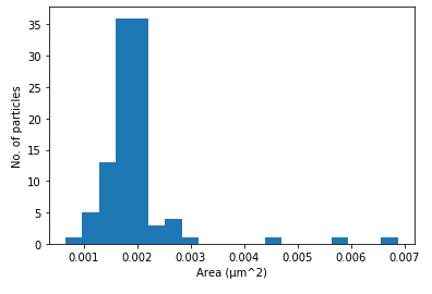
In the above code it is possible to plot particle area because this is automatically calculated in the particle_analysis function.

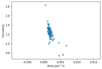
To plot a scatter plot of two properties you simply need to specify two properties in the arguments:

>>> particles.plot(['area','circularity'])

It is also possible to plot a 3D scatter plot of three properties by specifying three properties in the argument.

Plotting of more than one particle_list can be done using the top level plot() function:

>>> ps.plot([particles1,particles2],['area','circularity'])

All keyword arguments in matplotlib are available by passing them as arguments to the corresponding plotting function.

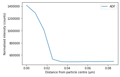
Plotting Radial Profiles

ParticleSpy provides the ability to plot a radial profile (that is an intensity profile from particle centre to edge) of image intensity or EDS signal intensity. A radial profile can be very useful for illustrating distributions in particles.

The following code shows how to plot a radial profile of image intensity.

>>> rp = ps.radial_profile(particle,['Image'],plot=True)

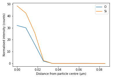
It is also possible to plot the intensity of certain elements from an EDS signal.

>>> rp = ps.radial_profile(particle,['Pt','Ni'],plot=True)

Saving Particle Images and Maps

In order to save images and maps of particles it is necessary to use Hyperspy’s save function.

>>> particles.list[0].image.save(filename)